Chapter 1 Getting to know R and RStudio
Goal
The main goal of this chapter is to facilitate you with the necessary tools and skills needed to begin working with R and RStudio.
What we shall cover
By the end of this chapter you should:
- know the difference between R and RStudio
- have R and RStudio installed on your PC
- have an understanding of what is meant by; R session, workspace/global environment, working directory, errors, warning and messages
- be able to work interactively with both R and RStudio
- be able to write reproducible scripts
- know what packages are and where to get them
- be conversant with R libraries and how to add them
- be able to install and load a package
Some Pointers on write-up
Blocked content (with grey/white background with grey border) are called R Chucks which are codes or commands written on a script. The # symbol indicates a comment usually used to give information about some line of code and ## indicates results or output of code which has been rendered/processed.
If you are not totally new to R, how about skipping to the Gauge yourself section and see what you need to brush up on.
1.1 What is R?
1.1.1 Defining R and tracing it’s history
R is many things, if you have never used a statistical package or are new to data analysis and indeed statistical programming (for whom these tutorials are geared towards), begin by viewing R as a calculator which can perform numerous analysis. If you have been using other statistical packages and more so if you were using the ‘drop-down-menu/click’ method, view R as your tool for reproducible analysis (a growing concern in publications and evidence based interventions in the development and humanitarian sectors).
More specifically, R is a statistical computing and graphics program. It is a dialect of S programming language developed by Ross Ihaka and Robert Gentleman in 1993. R is partly named after these two leading founder’s first names and partly in conformity to the “one-letter” names given to other programming languages developed at the Bell Laboratories of which S is one of them. The two founders developed the program while teaching at Auckland University in New Zealand. Their main aim was to offer their students a free statistical program they could use during their statistical class.
R as an implementation of the S programming language has much of the S code but with subtle difference, like lexical scoping which we shall discuss in detail in our follow-up book; R Beyond Essentials.
Over the years, R has grown from the little known statistical programming language used by a few university students in Auckland, to a widely used program applicable not only in academia, but also in other industries. It is currently being maintained by R's development core group. John Chambers, the founder of the S language is one of the core group members. Check out this page for current ratings for most statistical programs.
With the growing interest in R, there have been other programs developed with R as its base. Most of these are known as Intergrated Development Environment (IDE) that essentially help analysts and programmers to code more efficiently (IDE’s make R more user-friendly). The most widely used IDE’s include RStudio and Revolution Analystics. To distinguish R from the other programs, it is often called base R as it is the base for all the other programs. Just to clarify these two terms (base and IDE), you cannot have an IDE like RStudio without base R; base R is literally the foundation.
So in these tutorial series we shall refer to R as base R and we shall only work with RStudio, as it is suitable for an introductory session in R, it’s also as free as base R (but there is a commercial version).
1.1.2 Downloading and Installation of Base R
R is freely available for downloading from Comprehensive R Archives Network (CRAN). CRAN is R’s repository or a web server that stores identical and up to date version of its programs, codes and documentations.
1.1.2.1 Downloading the executable program
Before downloading, you will need to select one of CRAN’s mirrors. A mirror as the name suggests is a reflection (copy) of the original. In this case, there are numerous CRAN mirrors located around the world (you can select the one that is closest to you). The main purpose of these mirrors is to reduce network overload to the main server located at Institute for Statistics and Mathematics of WU (Wirtschaftsuniversit?t Wien), Austria.
Once you have selected a mirror, go ahead and click a suitable application for your operating system: Windows, Mac, or Linux. Next click “install R for the first time” and it should start to download the most current version of R.
1.1.2.2 Installing Base R
When downloading is complete, click on the executable program and then click run. This should take you through the following installation windows:
- A set-up language window where you choose the installation language you are most comfortable with.
- A welcome screen detailing the R version being installed. It is recommended you close all other running applications for a smooth installation.
- A license window which you can read before proceeding to the next installation window
- A window to indicate where R will be installed; the default is usually fine but you can change it if you are conversant with program installation and access.
- A window to select the components to be installed. The first component should be selected as it contains core files. The next two depend on your system, but R should be able to detect it.
- A start-up options window which you can either let R set or you can customize it. If you select to customize it, then you will get a window indicating the start up menu folder. Here you can choose the default to have it in the R folder or you can specify another location. You can also indicate that the start-up menu should not be created; however, it’s best to choose the default.
- Finally a window to indicate additional tasks to be performed during setup like creating a desktop icon, quick launch and registry files. If you will be using R often, you can click on the desktop or the quick launch options, but make sure to check the registry option as it is vital in R; and with that, installation should begin.
Checkout appendix 1 for a visual/snapshots guide on how to download and install R.
1.1.3 Tour of base R
Now that you have installed R, let’s get to know it. First locate the installed program either from the desktop, on the start menu or if on Windows clicking All Programs and search for R. Once you have located it, click on the program to start it. The first screen you see would look like this:
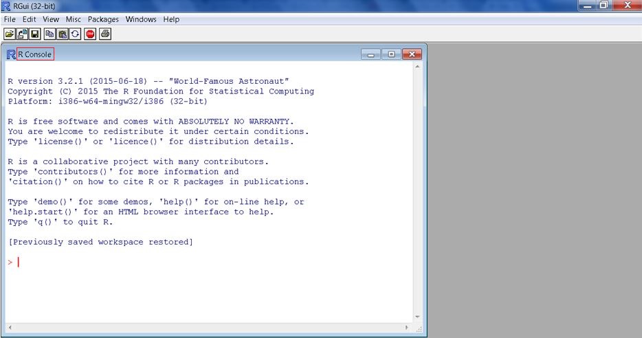
Base R
1.1.3.1 R at a glance
The first thing you notice are two windows; the main one with a menu bar and with a grey background and another window which has only the minimize, maximize and close buttons (an embedded window).
The embedded window is called the R Console and it’s R’s interactive platform for issuing commands (functions) which instantly produces an output similar to that of a normal calculator. The console is best suited for computations or expressions that fit in one line, something like addition, subtraction, multiplications, and divisions or any other simple computation. For multiple line computations like writing your own commands or functions, scripts are more suitable.
But before you get to type in your commands, there is an introductory message with information on R version installed, copyright issues, platform, warranty and conditions for use, R as a collaborative package, recommended citation and some start-up commands or functions.
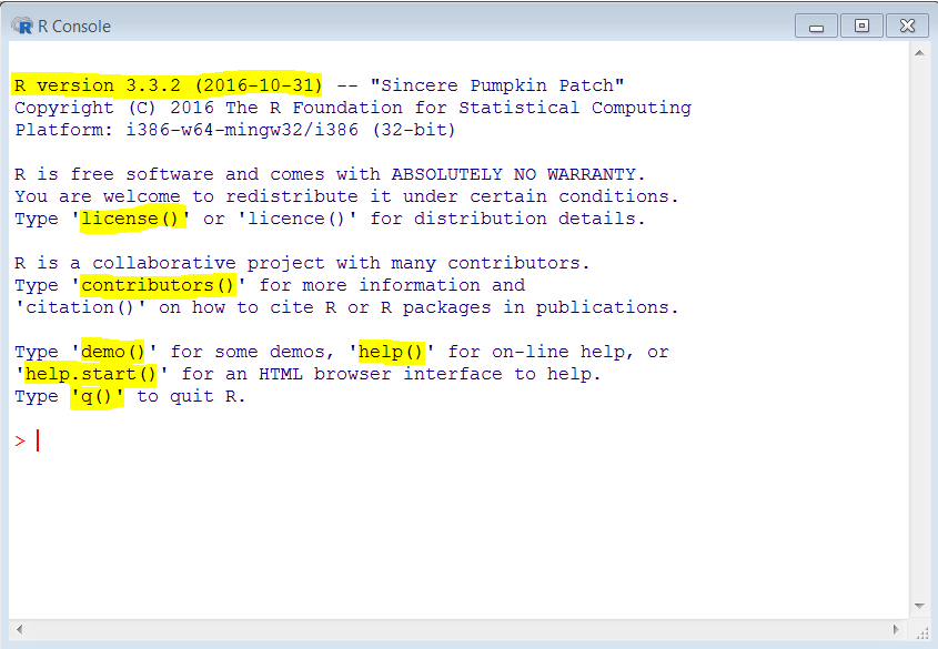
R’s introductory message on the console
Let’s explore some of these commands as an introduction to R’s console (interactive session) before we venture into the menu bar which discusses a number of issues about the console and other R windows. Commands are issued or typed right after the blinking cursor > (note, this can be changed later with the options function).
1.1.3.2 First interactive session on base R
One of the commands given in the introductory message is about the names of R contributors. Since R is a free program, it is generally developed and maintained by volunteers, for this reason it would be good to see some of the good people who have given us such a wonderful program for free. To do so, type contributors() and don’t forget the two parentheses () which indicate a command or a function call (as we shall soon learn).
## Type
contributors()
Hoping your first line of code worked. If it did, you should see a new window with some write-up on the contributors and a bit of history and inspiration that led to R’s development. If you received an error, please check your spelling and case: R is case sensitive, any slight misspelling would not yield expected results.
So now we can say we have written our first command on R: a great achievement. In R, writting commands is referred to as making a function call. We shall discussing function calls in chapter 2 but for now what you should know is that parenthesis in R indicate a function, therefore the word before the () is the name of a function. For example mean is a name and it is a function because it is followed by (). We say function call when you use a function or what you might call a command in other programs, for example when we use the mean function like this mean(c(2, 5, 6, 9, 3)), it means we have made a function call.
help.start() (please note the . between the two words). If you typed it correctly, then you will see a window titled Statistical Data analysis, below it are four subheadings namely manuals, references, miscellaneous materials and materials specific to your operating system. The help.start() function is a great reference point and you should consult it frequently as you learn R. I strongly advice you read the manual on Introduction to R alongside this book.
Word of encouragement, most of the details might not be clear right now as you have really not had a go at R, but after a few chapters you will be able to appreciate the details in these documents).
Two final commands that might be useful at this very early stage are clearing the console and quitting R from the command line.
Our console right now has quite a bit of information (introductory message, contributors() and help.start()), if you would like a blank/clear screen to type on, press control(Ctrl) + L and you should have a blank screen. Everything that was on the console should be cleared from the screen but not from history. R by default saves commands you issue and can be recovered from the history file. To quit R, you can either use the command line, click close from the menu bar or exit from file menu. To use the command line type q() on the console.
With that, we have successfully experienced R and are ready to do more, but first, we need to acquaint ourself with two other windows. The first isis called the workspace or the global environment and the other is script window.
1.1.3.3 R’s other core windows
1.1.3.3.1 The Workspace/Global Environment Window
As you get to work with R, you will soon discover that every entity in is referred to as an object; from the data to the functions.
To use any of this objects they need to be in an environment that R can access, this means for example that data has to be imported into R as well as functions to be used.
Initially the environment to which an R object is stored is called a workspace or the global environment. Objects are stored in this environment by creating variables (we will soon see how to create them), for instance, if you want to work with some data located in your computer, you must first bring it into R by creating a variable which will be temporarily stored on your workspace. This vairable would have a name for which you can use to carryout your analysis. This variable an object only available from the time you start working with R to when you logoff R; something referred to as an “R session”. To make a more permanent storage of variable or objects on your workingspace, they need to be saved to an R file with a “.RData” extension, that way, each time you log into R from the same folder/directory, R will make your data/objects available alongside commands used during that session.
In base R, the workspace/global environment is an invisible window whose content can be inspected by a call to objects(), or ls(). Try calling either of these two functions (objects/ls). At this point you should receive a character(0) output meaning there is no objects in your workspace. Later once we have learnt assignment operators you will be able to see your objects with this these functions or remove them with function rm().
1.1.3.3.2 The script window
When working interactively on the console, you are literally issuing commands without saving them. You can recall a function using a history file but sometimes you would want to have all the code in one prose which you can rerun some sections or all of it. R (and indeed many other programming languages) offers something called a script which is a text editor1 where you can write commands/codes; this is usually written in a new window called “R Editor”. A script written in this editor can be saved with a .R extension and can be retrieved later. Read more about scripting below.
1.1.3.5 R remembers
Every thing you do on the console or run from a script is temporary captured and stored by R. So if we do some computation/analysis, R will remember and retrieve it when needed. For example let’s compute the following on the console:
1 + 5
## [1] 6      Solution
10 + 102
## [1] 112    Solution
To recall any computation we use the “up” arrow key on the keyboard, we can also go forward with “down” arrow key. Using this feature we rerun commad/functions as they are or edit them as need be.
Commands which have been run are referred to as history and they are automatically captured by R in .Rhistory file. This history file (.Rhistory) is stored on your working directory and reloaded next time R is logged in from the same directory. Note, it is possible to tell R not to make these “.Rhistory” files, but it might not be a good idea for us right now.
1.1.3.6 R session
Before winding up this brief tour of R, it’s important to note one useful term that you will hear quite a bit of and that an R session. A session in R begins when you start-up R and ends when you close the program; this is important to know as it has certain implications. For example, everything you do during an R session is recorded or documented in a history file which as noted earlier can easily be stored and retrieved.
Note, quite a bit of this might not be clear right now, but it will definitely become clearer when we have defined some few variables or objects or simply when we have started working with R both at the console (interactively) or using a script.
Now let’s wind this section with a bit of computation on the console.
1.1.4 Base R’s console
Let’s use the console to do some simple computation similar to doing calculation on a standard calculator.
# Addition
2 + 5
## [1] 7
# Subtraction
4 - 10
## [1] -6
# Division
30/2
## [1] 15
# Multiplication
3 * 9
## [1] 27
Moving on, suppose we wanted to find even numbers or whether a number is divisible by another number. For example, what would you expect if you divided an even number with 2? Yes, indeed, you should get a whole number without any remainder or a point. An odd number would have a 0.5 remainder. Let’s test this:
# Even Numbers
#-------------
2/2
## [1] 1
4/2
## [1] 2
6/2
## [1] 3
20/2
## [1] 10
100/2
## [1] 50
100000000000000000000000000/2 # An even long number produces an exponent
## [1] 5e+25


# Odd numbers
#------------
5/2
## [1] 2.5
35/2
## [1] 17.5
37/2
## [1] 18.5
We can use this same logic, to compute divisibility of any number by another. If by dividing we get a remainder, then the number is not divisible by the other number. If on the other hand we got a full number without any remainder, then the number is divisible by the other. Let’s work it out on our new calculator (R console).
# Divisible numbers
#----------------
10/5
## [1] 2
100/20
## [1] 5
1700/17
## [1] 100


# Not divisible
#-------------
59/3
## [1] 19.66667
60/9
## [1] 6.666667
25/2
## [1] 12.5
70/3
## [1] 23.33333

# Try out other numbers
Now, that was good, but there is a way to quickly determine divisibility by using what is called modulo. Given two integers, modulo (indicated by two percentages %%) checks to see whether the integer on the left is divisible by the integer on the right. Modulo returns the remainder of the division such that if a number is divisible by another then we expect no remainder and therefore results to a zero.
For example, if we have 9 and 3, we could use modulo like this, 9%%3. In this case we are asking is 9 divisible by three?. So, if 9 is divisible by 3 then we expect a zero meaning there was nothing that remained after the division but if it were not the case, then we would expect to get the remainder of the division.
9 %% 3
## [1] 0
In Mathematics, 9 is referred to as the dividend and 3 as the divisor. If we had 9%%2 we expect a remainder of 1 where 9 is the dividend and 2 the divisor. When you divide 9 by 2 you get 4 and a remainder of one resulting in 4.5. In this case, the number 4 is referred to as the quotient and 1 the remainder. There is a whole discussion on this topic; but here I am merely introducing you to the concept which you could use in your programming.
Now let’s test it:
9 %% 3
## [1] 0

15 %% 7; 15/7
## [1] 1
## [1] 2.142857

# How about long numbers (at least one that you cannot figure out)
69294797 %% 8 # It says the remainder is 5
## [1] 5

# Let's confirm this
69294797/8 # Opps, we have a whole number, what is R up to?
## [1] 8661850

# R has default number of digits it can print, if your output exceed it like ours, then R will round it off to its default digit (in my case it is 7). To see your default:
getOption("digits")
## [1] 7
# and to change it
options(digits = 9)
# Now let's rerun our command
69294797/8 # we have our remainder (though not exactly 5 -- discussion for another session)
## [1] 8661849.62
Now, let’s briefly compute the mean (a measure of a data’s centrality) and see the number of ways we can do it.
What is the average of the following numbers?
        * 2, 5, 9, 3

            and

        * 5, 8, 10, 100
There are two ways you can do this (at least for a small amount of data), the first entails adding the values and then dividing with their totals just like a calculator, or the R way by using a function - mean().
#The calculator way
(2 + 5 + 9 + 3)/4
## [1] 4.75

#The R way
mean(c(2, 5, 9, 3))
## [1] 4.75
Notice that R’s way is simpler and can handle many numbers, however we had to enclose the numbers in parenthesis and a letter c at the front. “c” is a function that means combine (the values), combining values this way lets R treat the values as one unit rather than individual elements. We shall discuss this concept further during the vectorisation2 chapter.
I encourage you to get hold of some useful (numerical) data like the ages of your colleages/friends, class scores, hair/eye color in your area or some budget data and compute their average on the console. That should give you a good start to interacting with R.
At this point we have been able to make some few function calls, at least commands R understands and can get us results. But what if R does not understand what you are asking? Or what if R does not have the information needed, or there are either problems or other execution information? These are typical issues in any analytical program and there are ways of dealing with them. In R when these issues arise, we expect to receive an error a warning or a message. Let’s look at these terms as they would become quite frequent especially at this early stage.
1.1.5 Errors, Warnings and messages
1.1.5.1 Errors
Suppose you asked R to do something with a function that does not exist; like get an average of some data but you misspell the function name by typing means() instead of mean(). What do you think would happen?
means()R would go looking for what you have typed (means) and not what you meant (mean), so unless there is another function by that name, R would not find it. When this happens R would throw and error.
means()
#Error: could not find function "means"
An error therefore appears when R cannot find what you have asked it to get. Visualize it this way, you type in a command and hit enter; R then gets hold of your command and goes on a search for the description of the command or the actions the command should do. This search begins from your workspace followed by other areas called enclosing environments 3, the last of these environments being Base R, if the command is not found there, it hits the empty environment where no object exists and hence the error. The same process is followed by R when looking for data.
Note R literally stops the execution of the command and then sends you the error message: it’s a failure to launch scenario.
1.1.5.2 Warnings
What if you gave R a command it can find, but in this case you have used it incorrectly or there is a more effective command or simply put, there are potential problems with your function call. R would execute the command but issue a warning message indicating execution problems faced.
Key point here is that R will execute the function subject to the identified problems which it will detail as warning messages. For example, when you what to use an integer (as opposed to a numeric value), you have to tell R the value is an integer by using the letter L after the value. If you mistakenly add a decimal point before the letter L, then you will get a warning message.
# Unnessary use of a decimal point
1.L
## [1] 1
## Warning message:
## integer literal 1.L contains unnecessary decimal point

# Otherwise it should have been
1L
1.1.5.3 Messages
Messages are informative statements given with R output/results. They usually give information on how execution was performed, they do not signal a problem, just procedures used in execution.
For example, if there are missing values or method in a call, R can execute the function but issue a message indicating what value or method was used.
1.2 RStudio
R Studio is a more user friendly version of R, and one of R’s most growing and popular IDE’s. It includes a console, syntax-highlighting editor that supports direct code execution, as well as tools for plotting, history, debugging and workspace management “https://www.rstudio.com/products/rstudio/”.
Note we will be using RStudio for the rest of these tutorial series.
1.2.1 Downloading and Installing RStudio
To download the latest version of the program, go to RStudio and select a program suitable for your computer’s specification.
There is an open source and a commercial version running on Windows, Mac, or Linux. You can also get the desktop version of Rstudio or Server version. Read more on the differences and varieties of Rstudio here.
Read appendix 2 for details on how to download and install RStudio.
1.2.2 Getting to know RStudio layout
Once you have installed the program and clicked to start it, you will immediately notice four windows called panes.
Let’s begin with one pane you are now familiar with; the console (usually located at the bottom left, though it can be in any side).
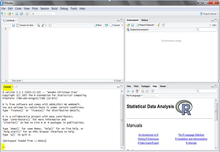
Rstudio Interface
You can start using it just as we did with base R's console and see if you can get the same results.
Right above the console is the script pane which is a scripting window. If you cannot see it, start a new script by clicking on files, then New File. For now select the first file type, R script, we shall discuss the other types of files in our next book (R - Beyond Essentials) and specifically on Chapter on Reproducible Analysis.
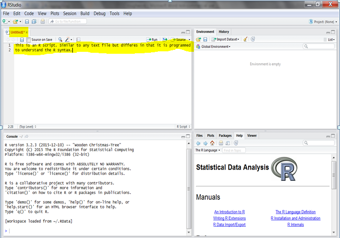
Rstudio Script Pane
On the top right side, is a window with two tabs, the first tab is called the environment and it is basically the workspace we discussed earlier. Next tab is the history window which captures commands and variables created during a session. These two tabs play an important role in storage and retrieval of your data and functions.
Below the workspace is a pane with five tabs. The first is the files tab which shows you the folders and files in the working directory. Next to it is the plotting window where graphs are displayed. The packages tab shows the packages/R extensions currently available on your system. Following the packages tab is the help tab where R’s help documentation is shown. Finally is the viewer tab, it is used to extend Rstudio to view internet local content more so related to applications such as Shiny which we will discuss in our second book “R - Beyond Essentials”.
With that quick tour of RStudio we hold any in-depth discussion on each tab, menu item or toolbar for our practice session.
1.2.3 Working with RStudio’s console
R Studio’s console is exactly like that of base R. To prove this, try and rework the exercises done on base R.
1.3 Installing and Loading Packages
A package is like a folder that contains grouped functions and/or data, this is what base R uses to store its functions and data. Read more about the packages that come with base R from the FAQ. Some of these packages form the core functions in R and others are recommended. You can also find information on all installed packages using the function installed.packages(). If you have more than one library you can specify a particular library by adding it’s path e.g. installed.packages(lib.loc = .libPaths()[1]).
In addition to the packages that come with base R, there are numerous other packages available from CRAN. These are packages with functions and data contributed by other R users: This is one of R’s distinguishing features - its extensibility. Anyone even you can add a package to R’s repository, as long as they are well coded.
When you start R, not all of the packages are available for use. The basic reason for this is to make R efficient in terms of memory usage and search. The packages that are automatically loaded are:
loadedNamespaces()
##  [1] "backports"  "bookdown"   "magrittr"   "rprojroot"  "graphics"
##  [6] "tools"      "htmltools"  "rstudioapi" "utils"      "yaml"
## [11] "grDevices"  "Rcpp"       "stats"      "datasets"   "stringi"
## [16] "rmarkdown"  "knitr"      "methods"    "stringr"    "digest"
## [21] "base"       "evaluate"
These are the core functions needed to make R operational. If you need to use any of the other unloaded base R packages, you need to tell R to make them available by using the function library. For example, you might want to do parallel computation for efficiency purposes; in R this can be achieved using the package parallel which is an R’s packages but by default not loaded.
library(parallel)Now let’s see if it is listed in the loaded packages.
loadedNamespaces()
##  [1] "backports"  "bookdown"   "magrittr"   "rprojroot"  "graphics"
##  [6] "parallel"   "tools"      "htmltools"  "rstudioapi" "utils"
## [11] "yaml"       "grDevices"  "Rcpp"       "stats"      "datasets"
## [16] "stringi"    "rmarkdown"  "knitr"      "methods"    "stringr"
## [21] "digest"     "base"       "evaluate"
The parallel package has been made available and can now be used. To read more about this package, make the following function call help(package = parallel).
If you need any of the contributed packages available on CRAN’s website, you will first need to install the package.
There are two ways of installing a package on either base R or RStudio, these are, graphical user interface (GUI) and the command line.
GUI Approach
- From
base R, go to thePackagetab thenInstall package(s).... You will then be prompted to select a mirror. Once that is done, you will be presented with a list of all packages, finish by selecting the desired package. Installation should begin immediately. - From RStudio, go to the
Packagestab located in the lower right pane then click theInstallicon. A dialogue box should open for you to specify the package needed but you will need to indicate the repository first. In addition toCRANthere are other R repositories like Bioconductor and Omegahat. In this tutorial, we shall only deal withCRAN, but feel free to explore the other repositories.
Command line approach
From the command line, you can download a package using the function install.packages() specifying the name of the package inside the parenthesis with quotation marks.
Before installing any package, let’s look at two issues related to loading and installation of packages, these are R search path and libraries.
1.3.0.1 Search Path
Earlier on we briefly mentioned R’s process of locating functions and data. For purposes of understanding packages available for use, let’s discuss search path some more (though not as concrete as we shall discuss it in “R- Beyond Essentials”).
The first question we want to ask ourselves is what is a search path? And the answer is; a search path is a sequence of locations that R follows as it “looks” for an object.
A subsequent question is, what is an object? Although we shall discuss this later, there is no harm knowing that everything in R is an object, from the commands or functions used, to the data and the output generated; packages are also objects. If an object is not on R’s search path, then R will throw an error, therefore, for one to use a package they need to “put” it on the search path by loading it. Loaded packages come second after the workspace/global environment. They comprise of the default packages already mentioned and any other loaded package. The search() function is used to determining the current search path.
# Current search path
search()
##[1] ".GlobalEnv"       "package:parallel   "tools:rstudio"  "package:stats"
##[5] "package:graphics"  "package:grDevices" "package:utils""package:datasets" ##[9] "package:methods"   "Autoloads" "package:base"
Notice that the parallel package is on the search path right after the global environment and right before the other packages? Now any function or data in any of these locations is available for use.
Recall, to make the package parallel available, we used the function library(), let’s expound on this.
1.3.0.2 Library
A library is a directory containing installed packages. Initially, there is only one library located at C:/Program Files/R/[R version]/library. In due time this location might become unwritable (hence cannot add more packages via install), in this case R might suggest you create another library. To do this .libPaths() function is used. “.libPaths” function can also be used to list the current libraries.
For example, we can create a new folder/directory and tell R to include it in its list of libraries.
# The current libraries
.libPaths()
## [1] "C:/Program Files/R/R-3.2.2/library"

# Create a new directory in R
dir.create("R/win-library/3.2")
# Create the new library
.libPaths("R/win-library/3.2")

# Confirm the new library is created
.libPaths()
## [1] "C:/Users/Hellen Gakuruh/Documents/R/win-library/3.2"
## [2] "C:/Program Files/R/R-3.2.2/library"
So now every time you install or load a package and you have more than one library, you can specify the library to use with the lib and lib.loc arguments. If this is not specified, then, R will automatically use the first library on the .libPaths().
Quite often with additional library(s), you might not know where a certain package is or which library has the package. In this case use the dir() function which lists files in a given directory.
# Listing packages in the new library directory
dir(.libPaths()[1])
##   [1] "acepack"          "assertthat"       "backports"
##   [4] "base64enc"        "BH"               "bitops"
##   [7] "bookdown"         "brew"             "caTools"
##  [10] "cellranger"       "chron"            "coin"
##  [13] "colorspace"       "crayon"           "curl"
##  [16] "data.table"       "DBI"              "DescTools"
##  [19] "devtools"         "dichromat"        "digest"
##  [22] "dplyr"            "evaluate"         "file10cc591e39e2"
##  [25] "file10cc7d741c3e" "file1a20e093962"  "file2dc17b843ef"
##  [28] "file2dc6c224780"  "fileefc5ffb3945"  "formatR"
##  [31] "Formula"          "gapminder"        "ggplot2"
##  [34] "ghit"             "git2r"            "gridExtra"
##  [37] "gtable"           "haven"            "highr"
##  [40] "Hmisc"            "htmlTable"        "htmltools"
##  [43] "httr"             "installr"         "ISLR"
##  [46] "jsonlite"         "knitr"            "labeling"
##  [49] "latticeExtra"     "lazyeval"         "lme4"
##  [52] "lmtest"           "magrittr"         "manipulate"
##  [55] "markdown"         "memoise"          "mgcv"
##  [58] "mime"             "minqa"            "modeltools"
##  [61] "multcomp"         "munsell"          "mvtnorm"
##  [64] "nlme"             "nloptr"           "nnet"
##  [67] "openssl"          "openxlsx"         "outbreaks"
##  [70] "packrat"          "PKI"              "plyr"
##  [73] "praise"           "pryr"             "pryr_0.1.2.zip"
##  [76] "R6"               "RColorBrewer"     "Rcpp"
##  [79] "Rcpp_0.12.3"      "Rcpp_0.12.3.zip"  "RcppEigen"
##  [82] "RCurl"            "readODS"          "readr"
##  [85] "readxl"           "reshape2"         "resumer"
##  [88] "rJava"            "RJSONIO"          "rmarkdown"
##  [91] "roxygen2"         "rprojroot"        "rsconnect"
##  [94] "rstudioapi"       "rvest"            "sandwich"
##  [97] "scales"           "selectr"          "sjmisc"
## [100] "stringdist"       "stringi"          "stringr"
## [103] "swirl"            "testthat"         "TH.data"
## [106] "tibble"           "tidyr"            "urltools"
## [109] "useful"           "vcd"              "whisker"
## [112] "withr"            "XLConnectJars"    "xlsx"
## [115] "xlsxjars"         "XML"              "xml2"
## [118] "yaml"             "zoo"
If you are wondering about the [1] after the .libPaths() function, it simply means get the first result from the output of .libPaths. This is a way of subsetting outputs which we shall be discuss later.
A little word of advice, the more you practice and use R, the more you will use add-on packages and most often than not, some of these packages will only be used once. To avoid loading your computer with numerous unused packages, consider installing them in a temporary directory. You need not create this folder as R starts one for every session and uses it to temporary store objects for the session. You can use this directory by calling on the tempdir() function.
Okay, now let’s practically apply these concepts by installing two packages. The first is a web scraping 4 package known as rvest and the other is a graphing package known as ggplot2. Let’s assume that we need rvest for only one session, but we will use ggplot2 frequently to plot graphs. Therefore, we will install rvest in a temporary directory and ggplot2 in the newly created library.
# Installing "rvest" to a temporary folder
install.packages("rvest", lib = tempdir())
Note, if you restart R, then the installation disappears and you will need to re-install the package.
# Installing a required package
install.packages("Rcpp")
# Installing "ggplot2" to one of the libraries
install.packages("ggplot2", lib = .libPaths()[1]) #or install.packages("ggplot2")
It would be useful for you to note that some packages come with other packages referred to as Imports. There are also those packages that a package depends on and other packages it suggests.
Always read the package’s documentation using help(package = "name")to know more about the package. An example is help(package = "rvest", lib.loc = temp()).
Now that the two packages are installed, they are still not yet on R’s search path. If you tried calling a function in one of these installed but unloaded packages you will receive an error.
# Calling a function from the installed "ggplot2" package which is not loaded
ggplot(x, aes(a, b)) + geom_point()
# Error: could not find function "ggplot"

search()
[1] ".GlobalEnv"        "package:parallel"  "tools:rstudio" "package:stats"
[5] "package:graphics"  "package:grDevices" "package:utils" "package:datasets"
[9] "package:methods"   "Autoloads"         "package:base"
To make them accessible to R, they need to be loaded by using the library() function. For the rvest package, remember to specify the library location, otherwise R would return a “not found” message.
# Loading rvest without specifying the library location
library(rvest)
##Error in library(rvest) : there is no package called 'rvest'

# First loading a depency that was installed in the same temp directory
library(xml2, lib.loc = tempdir())
# Now loading rvest by including the library location
library(rvest, lib.loc = tempdir())library(ggplot2, lib.loc = .libPaths()[1])
# Checking that they are loaded
search()
## [1] ".GlobalEnv" "package:ggplot2" "package:parallel"
## [4] "package:knitr" "package:stats" "package:graphics"
## [7] "package:grDevices" "package:utils" "package:datasets"
## [10] "package:methods" "Autoloads" "package:base"For practice, install and load a package called swirl. Swirl is an interactive learning platform that uses the console to teach a number of R topics. I highly recommend you start learning from swirl as soon as you are done with “R Essentials”, it will strengthen what we have discussed in preparation for our follow-up books: “R - Beyond Essentials” and “Introduction to Data Analysis and Graphics using R”.
1.4 Working directory
The working directory is a folder in your computer used to store all the files used or created during an R session. They help to organize your work and avoid scattering documents and programs.
For example, if you were working on different projects or tasks, like analyzing a survey at work, completing a schools assignment, or doing your household budget, then each one of these projects would have its own folder and any one of them would be your working directory whenever you are working on it. Therefore, your working directory will change depending on what project you are working on and it is best to tell R your working directory each time you start a new R session or switch projects or tasks.
There are two ways to tell R your working directory. Using the command line and using graphical user interface (GUI).
Using GUI:
- On Rstudio, go to the
Sessiontab and selectSet Working Directory. There are three possible locations:to source file location,to files paneand tochoose directory. The first location will set the working directory to the folder containing the R script, the next location will set the working directory to the files pane location which is your home directory. Lastly you can use thechoose directorylocation to select the folder to be used. - On base R, go to
file, thenChange Dir..., this should open a window where you can select the needed folder.
Using the command line (console):
First establish the full path to your working directory, then input that path to the setwd (set working directory) function.
But before setting the working directory, it is useful to find out your current working directory so you can know how to move to the new working directory. To do this, use the getwd (get the working directory) function.
# Current working directory
getwd()
##"C:/Users/Hellen Gakuruh/Documents"
My current working directory is my home directory often denoted by a ~ (tilde), however, since we are working on “R Essentials” I would like to make it my current working directory. “R_Essentials” folder is located within another folder called "Data Mania Inc" in my home directory, that is ("~/Data Mania Inc/Data_Mgt_Analysis_and_Graphics_R"). Note, folder names with spaces need to be in paranthesis (although it might be good to create folders without spaces, use “_" or “-” instaead of a space)
setwd("./Data Mania Inc/R_Essentials")Note, the easiest method for setting a working directory is using the GUI.
1.4.1 Introduction to scripting (reproducible analysis)
So far we have been using the console to produce instant outputs. This method of analysis is quick and easy when doing single line computation but it is not ideal for multiple analysis with more than one line of code. In addition, you might find it challenging later to reproduce the analysis (something that is gaining a lot of importance in publications). A good solution to this is working with scripts which are text files similar to notepad but programmed with syntax detection.
The script is used to type commands (functions and expressions) just as you would on the console. The difference is that on a script, codes do not generate instant output, instaed, one must click run for codes to be executed.
In addition to re-usability, another advantage of using scripts rather than the console is the ability to add short descriptions or explanations referred to as comments. Comments are added to help us understand our code in the future or guide other interested person(s) understand our code. Comments start with number sign/hash/pond sign # and any time R comes across it, it will disregard everything else on the same line as the hash tag.
Since we have not covered data object creation, we will create a short script generating our data on the fly and doing some bit of analysis on it. Basically, the script should be self explanatory given the comments used.
First open a new script (if none is opened), then type in the commands below.
# Combining the data elements
c(2, 5, 9, 3)
# Computing the sum
sum(c(2, 5, 9, 3))
# Getting the total number of elements in the dataset
length(c(2, 5, 9, 3))
# One way of computing the mean
sum(c(2, 5, 9, 3))/length(c(2, 5, 9, 3))
# Another way of computing the mean
mean(c(2, 5, 9, 3))
# Computing the median
median(c(2, 5, 9, 3))
# Conclusion: The median gives a better description of the average for this dataset
To get their output, click Run Selected, Re-Run Previous or Run Region from RStudio’s Code menu. A script can also be rendered by Run icon locates on the Script editor’s toolbar.
To save your script, go to the file tab and select Save As, and the script will be saved with .R extension.
Gauge yourself
Do you have the expected tools and skills from this chapter?
- Where can you download base R?
- How many windows does default R start-up have?
- What is a console?
- What do these () mean?
- How can you clear the console?
- What is a script and why would you use it?
- What is RStudio and how does it differ from R
- True or False, RStudio can be downloaded from CRAN
- How many panes does default RStudio have?
- What is your understanding of the following terms
- Mirrors
- Workspace/Global Environment
- R session
- Working directory
- Search path
- Error
- Warning
- Message
- What are packages
- How can you determine installed packages in any library?
- Which of the pre-installed packages are on search path?
- What is meant by a library?
- How can you install a package
- Are installed packages ready for use?
You are ready for the second chapter if you know these
- You can download base R from One of CRAN’s mirrors
- Default base R has 2 windows, the main window and an embedded R console
- A console is an interactive platform for data analysis
- Parenthesis () signify a function call
- On windows clr+L will clear the console
- A script is a text editor for writing code. It’s useful for multiple line of code and it’s reproducibility (re-usability) ability
- RStudio is an Integrated Development Environment (IDE) which makes coding in R much easy. It differs from base R in the sense that it is only functional when base R is installed, base R is it’s foundation
- False, the best way to download RStudio is from RStudios website
- Default RStudio has four panes each having multiple tabs
- Understanding of terms
- A mirror a copy of an original used to reduce network overload to the main server
- A workspace or global environment is a temporary storage environment
- R session begin when you start R and ends when you close the program
- A working directory is a folder in the computer with documents used or saved during an R session
- A search path is a sequence of location R goes through to locate an object. It begins from the workspace and ends at the empty environment
- An error occurs when R cannot locate an object. Execution of the command is halted and no results are given only the error message; R simply cannot execute the function
- Warning is issued to document potential problems which are numerous like using the wrong statistical method say chi-square for expected values less than five or invalid input say
1.Linstead of1Lfor integers. These messages are not fatal and R will execute the command but issue the warning message detailing problem in execution - Messages are used to give more information on how an execution was performed, they do not signal a problem. For example, they can be issued to show what method or value was used when if it not included in a call
- Packages are collection of functions and data bundled together to enable certain operations like specialized analysis or performance
- You can determine installed packages using the installed.packages() function. You can also specify a library installed.packages(lib.loc = .Library)
- Packages on the search path can be determined with loadedNamespaces()
- A library is a directory containing installed packages. The default library can be accessed with .Library. You can add other libraries with .libPaths()
- Packages are installed either through graphical user interface (GUI) or with the function install.packages(). The package name is included between the parenthesis in quotation marks e.g. install.packages(“ggplot2”)
- No, installed packages need to be loaded with the function library(), this time the name of the package is not quoted e.g. library(ggplot2)
Something Exra for you to find out on your own (not in notes)
- What do double quotation marks mean and do they differ from single quotation marks. Also find out when they are used. Tip read ?Qoutes
A text editor is a program used to write plain text for things like program source or configuration code. They differ from your usual word processors as they do not allow formating. Good example is Windows notepad.↩
Vectorisation is an operation carried out on an entire vector. A vector in R as we shall soon learn is an a data object containing zero or more elements. When there are more than one element, they must first be combined together so that they are treated as one object or vector for example c(2, 5, 9, 3).↩
In very simple terms, an environment in R is a location it searches for objects. This is usually applied in relation to function calls which could have several environments beginning with the function itself followed by the global environment. There is some sort of hierachy to these environments in terms of how objects are searched, these form some sort of tree like structures: We shall discuss this in greater details in our follow-up book (“R - Beyond Essentials”).↩
Web scraping is a term used to refer to reading and importing web-based data. Web scraping is also known as web harvesting or web data extraction.↩